Time-Series Databases for IoT & Monitoring: Explained with Examples

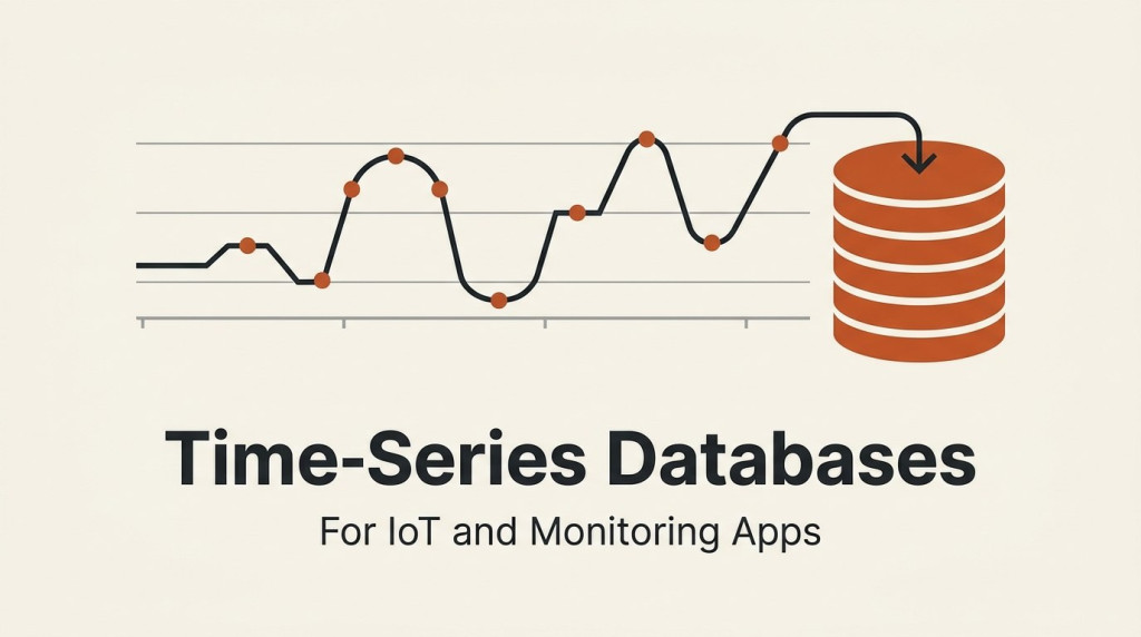
If you have ever wired up a fleet of sensors or stood up a monitoring stack, you know the feeling. The data never stops. A single temperature sensor reporting every 30 seconds is 2,880 rows a day. Put 500 of them in the field and you are writing over 1.4 million rows every single day, forever. Your CPU metrics, request latencies, and error counts behave the same way. It is a firehose, and it only points one direction: append.

Regular relational databases can technically hold this data. The problem is what happens next. Queries slow to a crawl, storage balloons, and the “delete everything older than 90 days” job locks your table for minutes. That is the moment most teams discover time-series databases.

This article explains what a time-series database (TSDB) actually is, when you need one, and then walks through a hands-on setup with TimescaleDB that you can run yourself in about 10 minutes. Every command below was run on a fresh install before publishing, so what you see is what you get.

What makes data “time-series”

Time-series data is any data where the timestamp is the primary axis. Each record is a measurement at a moment in time, and you almost always care about it in time order or time ranges. Think:

• IoT sensor readings (temperature, humidity, voltage, GPS position)
• Application and infrastructure metrics (CPU, memory, request rate, latency)
• Financial ticks, energy meter reads, vehicle telemetry

Three traits set this data apart from the customer records and orders your app usually stores:

1. It is append-heavy. New rows arrive constantly. Old rows almost never change.
2. It is queried by time window. “Average temperature per hour for the last day” is far more common than “find one specific reading.”
3. It ages out. Raw per-second data is precious for a week, useful for a month, and mostly noise after a year. You want to roll it up and then throw the raw data away.

A time-series database is built from the ground up around these three traits. That is the whole pitch.

Why your regular database struggles

You can absolutely start with plain PostgreSQL or MySQL, and plenty of small projects never need more. But as the row count climbs, a few things break down:

• Indexes get huge. A B-tree index over a billion-row table is expensive to keep in memory, and every insert has to update it.
• Time-range queries scan too much. Without time-aware partitioning, “last 6 hours” may still touch the whole table.
• Deletes are painful. Dropping old data row by row generates enormous write load and bloat.
• Storage is not optimized. Row-based storage cannot exploit the fact that consecutive sensor readings barely change.

Time-series databases fix each of these with time-based partitioning, columnar compression, and built-in data lifecycle tools. Let us see it in practice.

When you need one, and when you don’t

Reach for a time-series database when you have high-volume, timestamped, append-mostly data and you query it by time ranges or aggregates. Monitoring, IoT, and analytics dashboards are the classic fits.

You probably do not need one when your data is low volume, gets updated in place a lot, or is primarily relational (users, invoices, permissions). Do not migrate your whole app to a TSDB. The common and sensible pattern is to keep your business data in your main database and send only the metrics stream to a time-series store.

The landscape

A few options you will run into:

• TimescaleDB is a PostgreSQL extension. You get real SQL, joins, and the entire Postgres ecosystem, plus time-series superpowers. Great when your team already knows SQL.
• InfluxDB is a purpose-built TSDB with its own query languages. Popular in pure IoT and metrics setups.
• Prometheus is a monitoring system with a built-in TSDB, tuned for scraping infrastructure metrics. It is usually a target, not a general database.
• ClickHouse is a columnar analytics database that many teams push time-series workloads into at very large scale.

For this walkthrough I picked TimescaleDB, because if you know SQL you already know 90 percent of it, and you can run it anywhere Postgres runs.

Hands-on: TimescaleDB in about 10 minutes

You need Docker installed. That is the only prerequisite.

1. Start the database

docker run -d --name tsdb-demo -p 5432:5432 \
  -e POSTGRES_PASSWORD=tsdemo123 -e POSTGRES_DB=demo \
  timescale/timescaledb:latest-pg16

If port 5432 is already taken on your host, map a different one (for example -p 5433:5432). Give it about 20 seconds, then open a shell into it:

docker exec -it tsdb-demo psql -U postgres -d demo

2. Turn on TimescaleDB

Inside psql:

CREATE EXTENSION IF NOT EXISTS timescaledb;

3. Create a normal table

Nothing special yet. This is a plain Postgres table.

CREATE TABLE sensor_data (
  time        TIMESTAMPTZ      NOT NULL,
  device_id   TEXT             NOT NULL,
  temperature DOUBLE PRECISION,
  humidity    DOUBLE PRECISION
);

4. Convert it into a hypertable

This is the key step. A hypertable looks and behaves like one table, but underneath TimescaleDB automatically splits it into “chunks” partitioned by time. Here we use one-day chunks.

SELECT create_hypertable('sensor_data', by_range('time', INTERVAL '1 day'));

 create_hypertable
-------------------
 (1,t)

Every insert now lands in the right time chunk automatically, and time-range queries only touch the chunks they need.

5. Load some data

Let us simulate 3 devices reporting every 30 seconds for 14 days. Postgres can generate that for us.

INSERT INTO sensor_data
SELECT ts, d.device_id,
       21 + 8*sin(extract(epoch FROM ts)/86400) + random()*0.5,
       55 + 15*cos(extract(epoch FROM ts)/86400)
FROM generate_series(now() - interval '14 days', now(), interval '30 seconds') AS g(ts)
CROSS JOIN (VALUES ('sensor-a'),('sensor-b'),('sensor-c')) AS d(device_id);

That gives us a realistic pile of data:

SELECT count(*) AS rows, pg_size_pretty(hypertable_size('sensor_data')) AS size
FROM sensor_data;

  rows  | size
--------+-------
 120963 | 12 MB

6. Query by time bucket

Here is where time-series databases shine. The time_bucket function groups rows into fixed windows, which is exactly how you feed a dashboard. This asks for the hourly average temperature per device over the last 3 hours:

SELECT time_bucket('1 hour', time) AS bucket, device_id,
       round(avg(temperature)::numeric, 2) AS avg_temp
FROM sensor_data
WHERE time > now() - interval '3 hours'
GROUP BY bucket, device_id
ORDER BY bucket DESC, device_id;

         bucket         | device_id | avg_temp
------------------------+-----------+----------
 2026-08-05 19:00:00+00 | sensor-a  |    15.05
 2026-08-05 19:00:00+00 | sensor-b  |    15.09
 2026-08-05 19:00:00+00 | sensor-c  |    15.11
 2026-08-05 18:00:00+00 | sensor-a  |    14.94
 ...

Plain SQL, but time-aware and fast because it only scans the recent chunks.

7. Pre-compute rollups with continuous aggregates

Running that time_bucket query over a year of raw data on every dashboard refresh would be wasteful. A continuous aggregate is a materialized rollup that TimescaleDB keeps up to date for you in the background.

CREATE MATERIALIZED VIEW sensor_hourly
WITH (timescaledb.continuous) AS
SELECT time_bucket('1 hour', time) AS bucket,
       device_id,
       avg(temperature) AS avg_temp,
       max(temperature) AS max_temp,
       min(temperature) AS min_temp
FROM sensor_data
GROUP BY bucket, device_id
WITH NO DATA;

Tell it to refresh itself every hour:

SELECT add_continuous_aggregate_policy('sensor_hourly',
  start_offset      => INTERVAL '3 days',
  end_offset        => INTERVAL '1 hour',
  schedule_interval => INTERVAL '1 hour');

Materialize the existing data once, then query the rollup instead of the raw table:

CALL refresh_continuous_aggregate('sensor_hourly', NULL, NULL);

SELECT bucket, device_id, round(avg_temp::numeric, 2) AS avg, round(max_temp::numeric, 2) AS max
FROM sensor_hourly
ORDER BY bucket DESC, device_id
LIMIT 3;

         bucket         | device_id |  avg  |  max
------------------------+-----------+-------+-------
 2026-08-05 19:00:00+00 | sensor-a  | 15.05 | 15.31
 2026-08-05 19:00:00+00 | sensor-b  | 15.09 | 15.37
 2026-08-05 19:00:00+00 | sensor-c  | 15.11 | 15.34

Your dashboard now reads from a small, pre-aggregated table no matter how big the raw data gets.

8. Compress old data

Old chunks rarely change, so you can store them in a compressed columnar format. Configure it, then compress the chunks older than a day:

ALTER TABLE sensor_data SET (
  timescaledb.compress,
  timescaledb.compress_segmentby = 'device_id',
  timescaledb.compress_orderby   = 'time DESC'
);

SELECT add_compression_policy('sensor_data', INTERVAL '7 days');

Here is the payoff, measured on this exact dataset:

SELECT pg_size_pretty(sum(before_compression_total_bytes)) AS before,
       pg_size_pretty(sum(after_compression_total_bytes))  AS after,
       round(sum(before_compression_total_bytes)::numeric /
             NULLIF(sum(after_compression_total_bytes), 0), 1) AS ratio_x
FROM hypertable_compression_stats('sensor_data');

 before |  after  | ratio_x
--------+---------+---------
 10 MB  | 2544 kB |     4.2

A 4.2x reduction on this small, slightly noisy sample (the raw size shows as 10 to 11 MB depending on the run, since the sample data is randomized). On real production tables with more columns and smoother signals, 10x or more is common. The compression policy you added will now do this automatically for any chunk older than 7 days.

9. Expire raw data automatically

Finally, tell the database to drop raw data older than 90 days so it never grows without bound:

SELECT add_retention_policy('sensor_data', INTERVAL '90 days');

You can see all the background jobs you just created:

SELECT job_id, application_name, schedule_interval
FROM timescaledb_information.jobs
WHERE application_name NOT LIKE '%Telemetry%'
ORDER BY job_id;

 job_id |              application_name              | schedule_interval
--------+--------------------------------------------+-------------------
      3 | Job History Log Retention Policy [3]       | 06:00:00
   1000 | Refresh Continuous Aggregate Policy [1000] | 01:00:00
   1001 | Columnstore Policy [1001]                  | 12:00:00
   1002 | Retention Policy [1002]                    | 1 day

Three of those are the policies you just set up: refresh the hourly rollup, compress week-old chunks, and drop 90-day-old raw data. The database now maintains itself.

What you just gained

In under 10 minutes and without leaving SQL, you built a data pipeline that:

• ingests high-frequency readings into time-partitioned storage,
• answers time-window queries fast,
• keeps pre-computed rollups fresh for dashboards,
• compresses aging data to a fraction of its size,
• and expires raw data on a schedule.

Doing all of that on a plain relational table would mean manual partitioning, cron jobs, and a lot of custom code. That is the practical difference a time-series database makes.

Production gotchas worth knowing

• Pick your chunk interval with care. Aim for chunks that hold a manageable slice of data, roughly a few days for most workloads. Too small and you get thousands of tiny chunks; too large and compression and retention get coarse.
• You cannot cheaply update compressed data. Compression assumes old data is immutable. If you need late-arriving corrections, account for that before you compress.
• Continuous aggregates lag by design. The end_offset keeps the most recent, still-changing window out of the rollup. For live “last 5 minutes” panels, query the raw table and use the aggregate for everything older.
• Keep business data separate. Send metrics to your TSDB, keep users and orders in your primary database, and join only when you truly need to.

Where to go next

Point your existing metrics agent (Telegraf, a Prometheus remote-write endpoint, or your own app) at this database and swap the synthetic data for real readings. Wire Grafana on top for dashboards. The schema and the policies you built here carry over directly.

Time-series data is one of those problems that looks manageable right up until it isn’t. Setting up the right tool early, before the firehose turns on, saves you a painful migration later. And as you saw, the barrier to starting is basically one docker run and a handful of SQL statements.